Convolutional Nets
Felix Bogdanski, since 23.3.2018
In the article Artificial Neural Networks we designed, trained and evaluated a fully connected, dense neural network. While purely dense nets are suitable tools for many data structures, at times it is their density which can be a little too much. In this article, we introduce a technique called Convolution to not only tame the neural connectivity of dense nets, with respect to the hardware limits we currently have, but also enhance the representational power for high dimensional data, such as images or audio.
Density Reduction
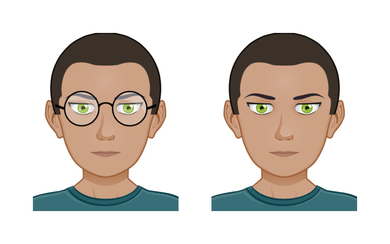
Bob is a good coder, he spends significant amounts of time in front of a screen. He wears his glasses when he works after all these years. Bob does not want to be disturbed being in a concentrated state, therefore we are interested to detect when he wears them.
An image comes in with three color channels (RGB), which gives in total to sense. The raw net output will be softmaxed under a negative log-loss cross-entropy regime, using both classes as training targets for classification.
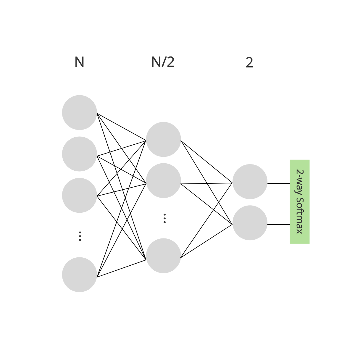
If we use a dense net with layout and the image flattened into a vector, we would need weights. A single float number takes 4 bytes on the JVM, so this amount would take roughly 429 GB of RAM. The current high-end GPUs used for visual recognition offer about 24 GB RAM, so we have to reduce the amount of weights. If we cut out the middle layer to have , which is the smallest layout possible, we would need weights, roughly 4 MB of RAM, which is a manageable size. Imposing a bottleneck, which leads to a simple representation of the input, can be used to reduce weights, indeed, if the model responds well to the drastic narrowing. However, it is obvious that dense layers and high resolution data quickly escalate the Curse of Dimension and it is not guaranteed that bottlenecks always work.
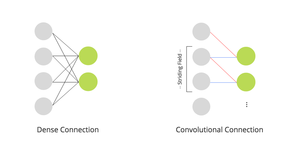
The vector on the left is fully connected, leading to ,
whereas the vector on the right is convoluted with
Another approach to reduce the amount of weights is to use a convolutional layer. While the philosophy of a dense layer is to fully wire a fixed amount of in- and output neurons (), a convolutional layer dynamically generates output neurons using a field of weights which is slid over the input with stride , generating a neuron per step. With this technique, we have more control over the output dimensions and the neural connectivity can be significantly reduced, while too generating a simple version of the input. A fun exercise to the reader is to draw different configurations of and to express dense with convolutional layers. :-)
Extension to Tensor3D
Now we can convolute vectors to reduce the connectivity, but a vector may be cumbersome to describe our three-dimensional material world, therefore we are interested in extending the technique to the third dimension.
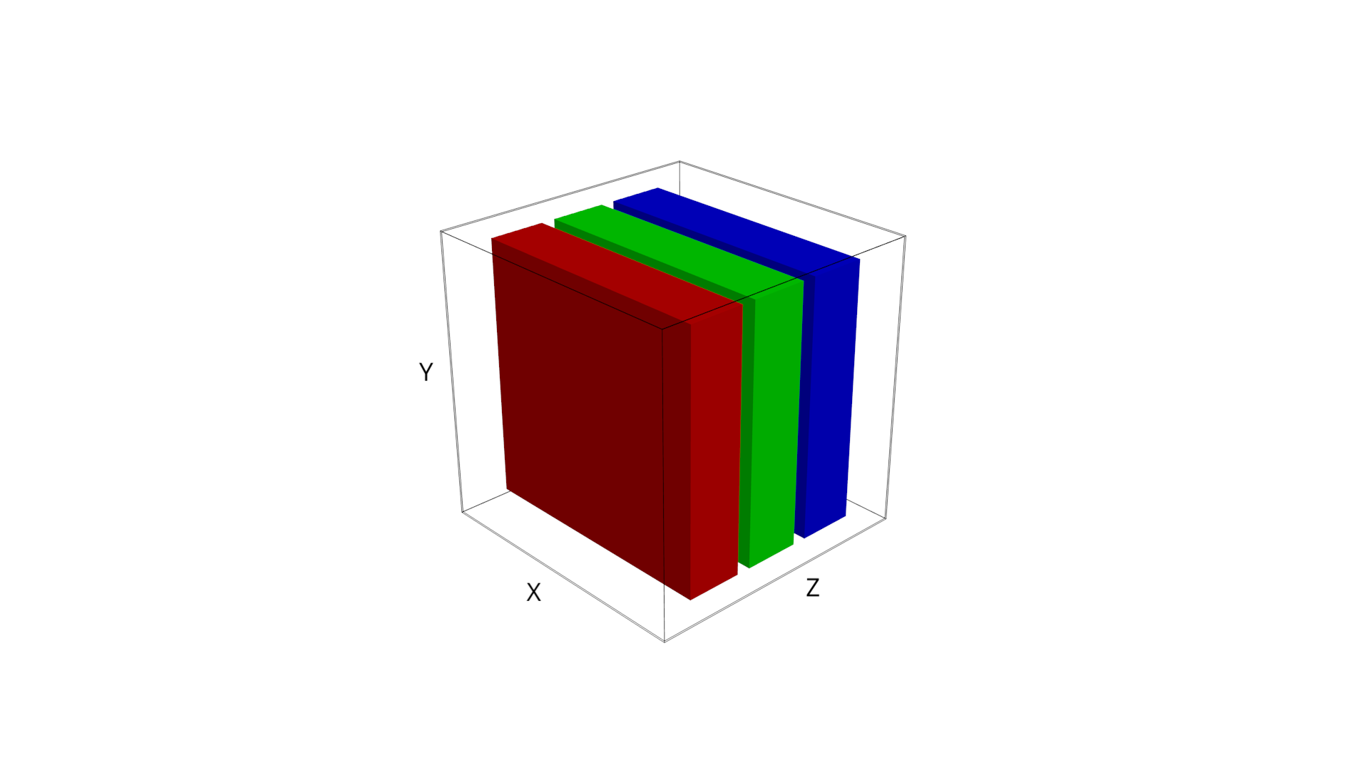
A can represent a color image, where RGB channels are bound to the axis.
Let us introduce , which is a cubic volume accessed by coordinate triple . A vector can be embedded in it, say vertically using shape , a matrix with shape and in our case, a RGB image of Bob with . The structure is versatile enough to represent other things from our material world, like sound spectra or mesh models.
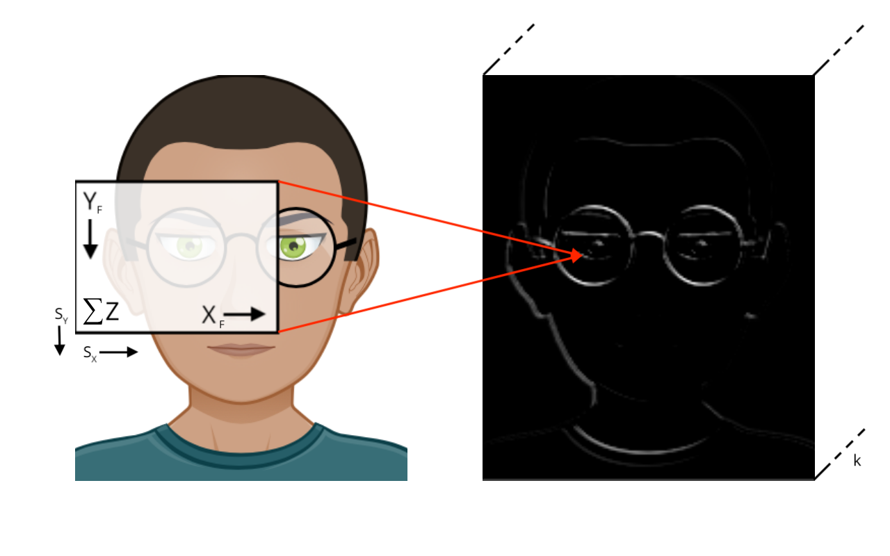
Each stride of weight field is convoluted to generate a unit in the output tensor, the input axis is up.
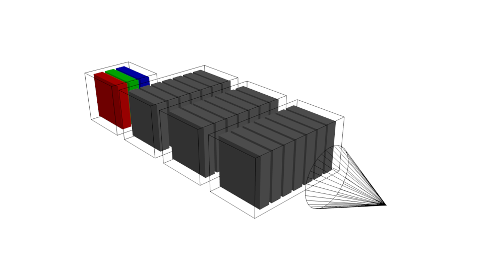
Multiple, independent weight fields can be attached to the input, generating a (deeper) tensor from it.
The convolution operator applied on a is much like the vectorial counterpart. The difference is, to generate the output, we slide the weight field over the input by dimensions and we add over the axis. The term Deep Learning refers to this additive depth of the input volume, since the whole input tensor is flattened into one layer of the output tensor, which possibly is even deeper than the input, depending on the number of independent weight fields attached. A weight field senses all dimensions of the input slice tensor with a dedicated neuron, leading to a number of learnable per field, and in total for the layer. The actual convolution of one of the input slice tensors and field tensor can be formulated by linearizing both tensors into matrices, , regularly multiplying them, while harnessing optimized linear algebra routines (BLAS).
Multiple convolutional layers can be stacked, usually ending with dense,
convolutional or averaging layers and a suitable loss function.
Now we can chain multiple convolutional layers, leading to architectures which learn more and more simple representations of the input, depending on length and depth of the chain. For visual recognition, the weight fields usually are small, e. g. , but numerous make it deep, and with a stride , the spatial size of the input can be gradually diminished along the way to the loss function, enforcing compression to highlight features of the respective class to be recognized.
Visualizing the Learnings
To understand what the convolutional layers actually do inside when learning different classes, we build a small architecture and visualize the activations per layer before and after training. Bob works with sharp minded people, and they all wear glasses, and they all don't want to be disturbed when wearing them, so we have a little more pictures for training.
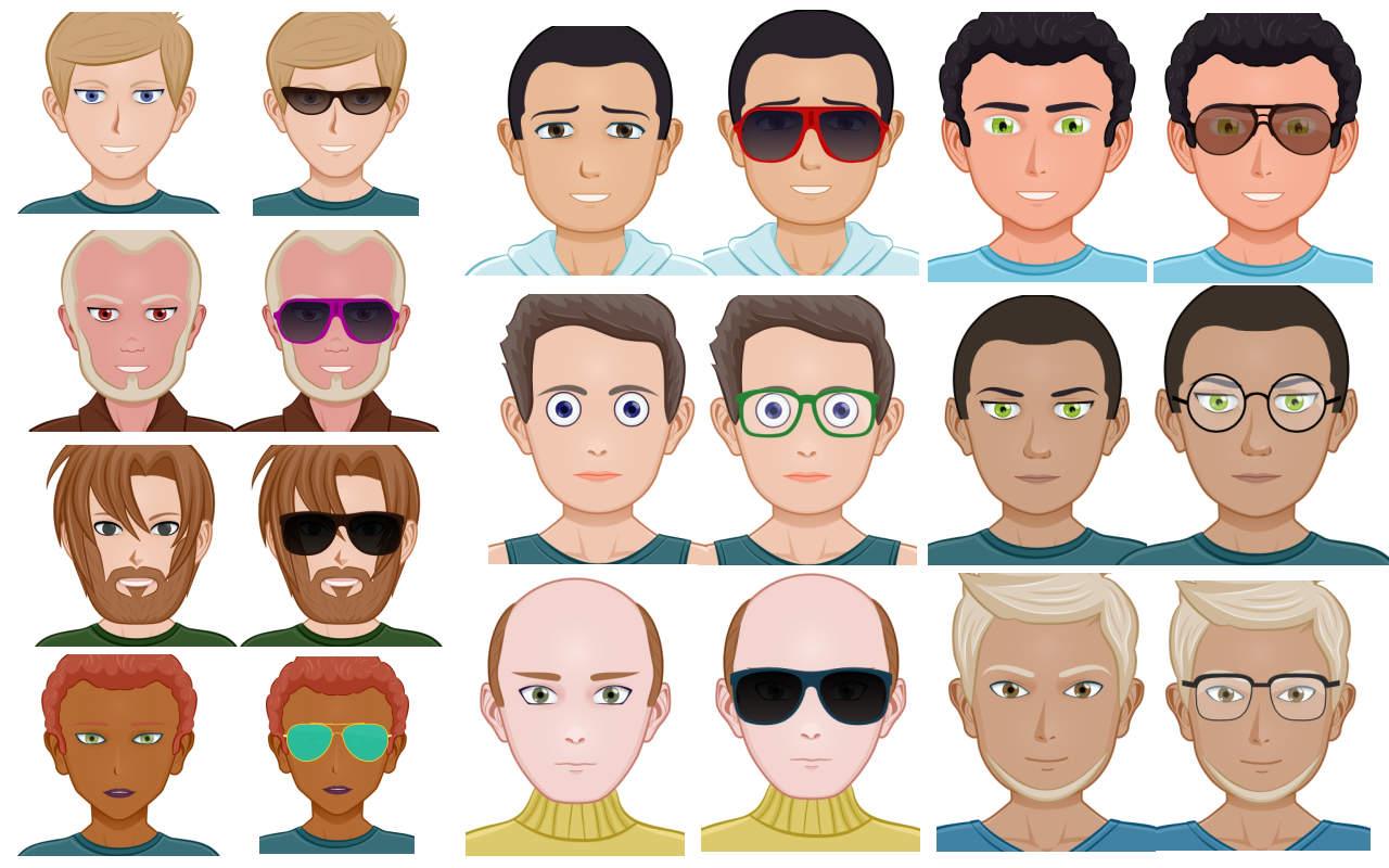
The good thing with these avatars is, the different classes are all perfect copies, except the eye region of course. We force the net to actually learn the differences between glasses and no glasses. Otherwise, for our little experiment, the net might lazily learn arbitrary edges to separate, which might not be related to our classification problem at all. This is often the case when the net has too much freedom for too few training samples.
Let us enter Scala land now. First, we load the PNG images of our avatars into tensors:
  import neuroflow.application.plugin.Extensions._
  import neuroflow.application.plugin.Notation._
  import neuroflow.application.processor.Image._
  import neuroflow.core.Activators.Float._
  import neuroflow.core._
  import neuroflow.dsl.Convolution.autoTupler
  import neuroflow.dsl.Implicits._
  import neuroflow.dsl._
  import neuroflow.nets.gpu.ConvNetwork._

  val glasses = new java.io.File(path + "/glasses").list().map { s =>
    (s"glasses-$s", loadTensorRGB(path + "/glasses/" + s).float, ->(1.0f, 0.0f))
  }.seq

  val noglasses = new java.io.File(path + "/noglasses").list().map { s =>
    (s"noglasses-$s", loadTensorRGB(path + "/noglasses/" + s).float, ->(0.0f, 1.0f))
  }.seq
The target class vectors are tupled with the images. Then, we find a simple layout under the softmax loss function:
  val f = ReLU

  val c0 = Convolution(dimIn = (400, 400, 3), padding = 1, field = 3, stride = 1, filters = 1, activator = f)
  val c1 = Convolution(dimIn = c0.dimOut,     padding = 1, field = 3, stride = 1, filters = 1, activator = f)
  val c2 = Convolution(dimIn = c1.dimOut,     padding = 1, field = 4, stride = 2, filters = 1, activator = f)
  val c3 = Convolution(dimIn = c2.dimOut,     padding = 1, field = 3, stride = 1, filters = 1, activator = f)

  val L = c0 :: c1 :: c2 :: c3 :: Dense(2, f) :: SoftmaxLogEntropy()

  val μ = 0

  implicit val weights = WeightBreeder[Float].normal(Map(
    0 -> (μ, 0.1),  1 -> (μ, 1), 2 -> (μ, 0.1), 3 -> (μ, 1), 4 -> (1E-4, 1E-4)
  ))

  val net = Network(
    layout = L,
    Settings[Float](
      learningRate    =  { case (i, α) => 1E-3 },
      updateRule      =  Momentum(μ = 0.8f),
      batchSize       =  Some(20),
      iterations      =  250
    )
  )

  /*
               _   __                      ________
              / | / /__  __  ___________  / ____/ /___ _      __
             /  |/ / _ \/ / / / ___/ __ \/ /_  / / __ \ | /| / /
            / /|  /  __/ /_/ / /  / /_/ / __/ / / /_/ / |/ |/ /
           /_/ |_/\___/\__,_/_/   \____/_/   /_/\____/|__/|__/
                                                              1.6.2


              Network : neuroflow.nets.gpu.ConvNetwork

              Weights : 80.061 (≈ 0,305408 MB)
            Precision : Single

                 Loss : neuroflow.core.SoftmaxLogEntropy
               Update : neuroflow.core.Momentum

               Layout : 402*402*3 ~> [3*3 : 1*1] ~> 400*400*1 (ReLU)
                        402*402*1 ~> [3*3 : 1*1] ~> 400*400*1 (ReLU)
                        402*402*1 ~> [4*4 : 2*2] ~> 200*200*1 (ReLU)
                        202*202*1 ~> [3*3 : 1*1] ~> 200*200*1 (ReLU)
                        2 Dense (ReLU)


           O O O O O O O O O O      O O O O O O O O O O
           O O O O O O O O O O      O O O O O O O O O O
           O O O O O O O O O O      O O O O O O O O O O      O O O O O      O O O O O
           O O O O O O O O O O      O O O O O O O O O O      O O O O O      O O O O O
           O O O O O O O O O O      O O O O O O O O O O      O O O O O      O O O O O          O
           O O O O O O O O O O      O O O O O O O O O O      O O O O O      O O O O O          O
           O O O O O O O O O O      O O O O O O O O O O      O O O O O      O O O O O
           O O O O O O O O O O      O O O O O O O O O O      O O O O O      O O O O O
           O O O O O O O O O O      O O O O O O O O O O
           O O O O O O O O O O      O O O O O O O O O O

  */
Our network is a shallow conv net, with a 2d-dense layer before the loss function, leading to 80.061 weights, which is a huge reduction, compared to the smallest dense net possible with 960.000 weights. Remember we want to enforce compression, so we attach only one filter per layer. The activator is often used with convolutional nets (we discussed it already). A little padding is added to keep output sizes even. Next, we need to get images out of the layers.
  def writeLayers(): Unit = {
    samples.foreach {
      case (id, xs, ys) =>
        val t0 = (net Ω c0).apply(xs)
        val t1 = (net Ω c1).apply(xs)
        val t2 = (net Ω c2).apply(xs)
        val t3 = (net Ω c3).apply(xs)
        val i0s = imagesFromTensor3D(t0)
        val i1s = imagesFromTensor3D(t1)
        val i2s = imagesFromTensor3D(t2)
        val i3s = imagesFromTensor3D(t3)
        i0s.zipWithIndex.foreach { case (img, idx) => writeImage(img, path + s"/c0-$idx-$id", PNG) }
        i1s.zipWithIndex.foreach { case (img, idx) => writeImage(img, path + s"/c1-$idx-$id", PNG) }
        i2s.zipWithIndex.foreach { case (img, idx) => writeImage(img, path + s"/c2-$idx-$id", PNG) }
        i3s.zipWithIndex.foreach { case (img, idx) => writeImage(img, path + s"/c3-$idx-$id", PNG) }
    }
  }
The focus does exactly this, it gives us the raw activations of a layer as tensor , and for each layer of , a grayscale PNG image is written to file. What does it look like for before training?
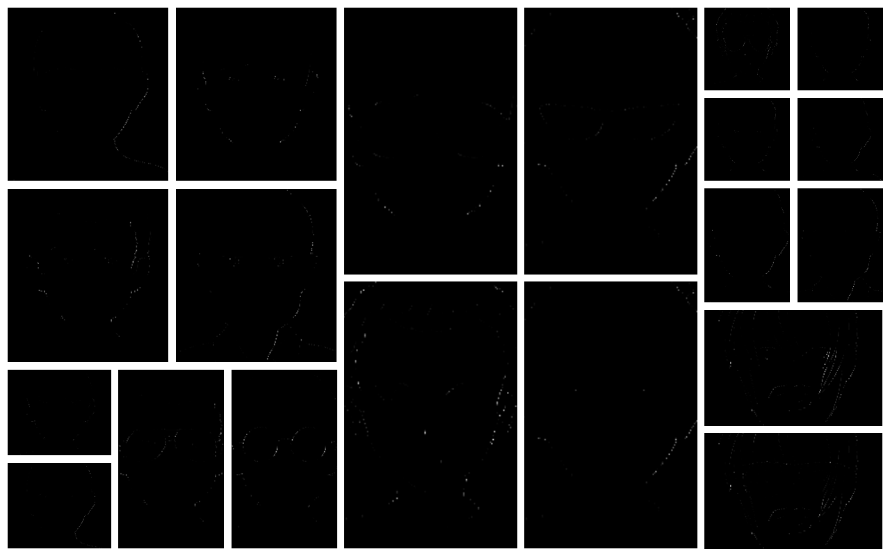
Not much to see here, the weights sum out each other, since we initialized them drawn from normal distribution with symmetry at . Now the net has all freedom to decide which regions are important for the classification. Then, we train for a few epochs and look again:
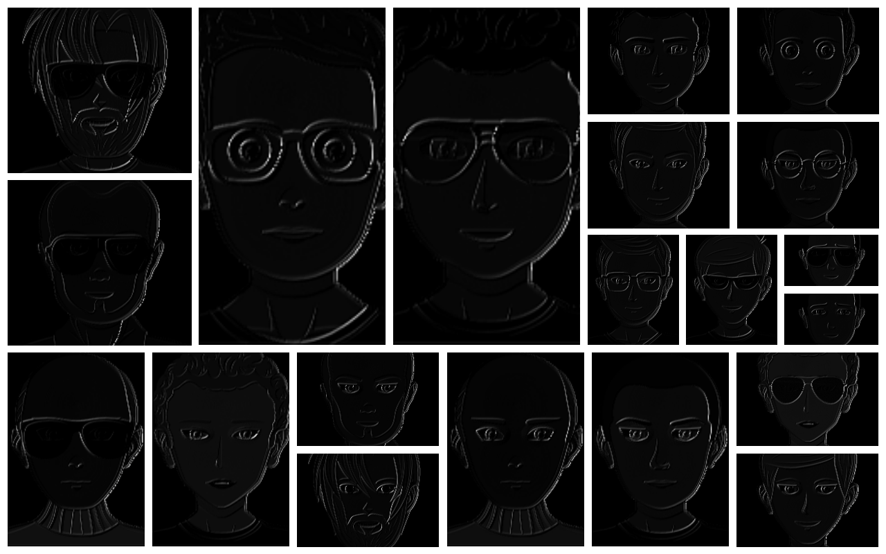
The net decided to highlight the eye region most. Sure, all regions are boosted by the weights since the size of the field is small and responsible for generating the whole output, but the average focus is on the eye region, compared to the neck, mouth, nose and forehead regions. This simplification makes it easier for the last fully connected layer to decide whether the input wears glasses. When it comes to images, a convolutional network is a graphical filter capable of learning.
Representational Power
When I first heard about the curse of dimensionality dense neural networks bring, I thought that it might be only a matter of time until more powerful parallel processing units with enough of memory would be available, to overcome these limits. I think of a Quantum Processing Unit (QPU), with which I could train large images and other high dimensional data, using nothing but purely dense nets. I like the idea, because I find them a little more plausible on the biological level, e. g. why would a lazy organism chop and copy inputs several times, like the convolution operator does?
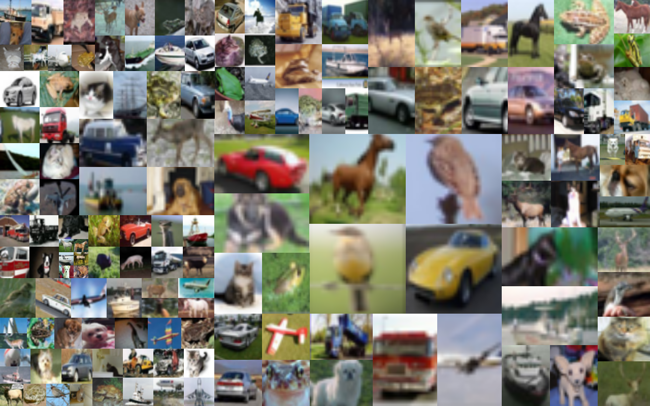
The CIFAR set has 50.000 color images for training and 10.000 for testing from 10 classes á and is a fast benchmark,
since deep models (>1 million weights) can be trained in a few hours on a Tesla P100 or a 1080Ti.
So I started experiments with the CIFAR set and pure dense nets, and it seems there is a natural limit for dense nets when it comes to generalization on high dimensional data under a bottleneck. A dense net would be able to perfectly learn all 50k training images, but I couldn't get the recognition rates beyond 50 % on the test set. The size of the bottleneck was not really important, I tried several configurations, with as much weights as my GT750M would allow. Pictures were not enhanced in pre-processing steps. Instead, with a 9-layer deep convolutional network from scratch, I could get the rates over 70 % for the test set, which is decent. I only know of dense nets with heavily pre-processed CIFAR images (contrast enhancing et al), which get close to this region. Conv nets, which are tuned by teams to the CIFAR challenge with up to 1000 layers, are somewhere in the 9X% area. My experiment shows that convolutional layers learn simple representations of features, like a graphical preprocessor or filter, and therefore have more representational power for high-dimensional data than dense nets, otherwise they couldn't be better on the raw, unenhanced test set, at least with the hardware we currently have. As a musician, I am interested in audio stuff too, so let's see what's next. (Spiking Neural Nets? :o))
Thanks for reading.