Artificial Neural Networks
Felix Bogdanski, since 1.7.2016
Wolves have paws and jaws, birds feathers, the universe toroids, and we humans, well, we have our brain to build machines. Machines, capable of doing tedious tasks we no longer want to do, or to increase productivity, et cetera. We have been there before, back in industrialization times, and face a similar situation today, but in a more virtual, digital world. The machines we seek to build should have functionality, which is rather found in brains than muscles, e. g. recognizing patterns in data. Because our brain is a purely natural tool, it is a good blue print, so we study the structure behind this organic intelligence and use it to create such machines. I think that we will never understand our brain entirely intellectually, because this kind of understanding comes from within the brain itself. Limited beings we are, aren't we? However, we can get close to human intelligence — as long as we are very precise about the task, our expectations and have enough examples to learn from.

There is a rich green, vigorous ginseng bonsai tree in my office. Every time I look at it, my brain fires with other pictures, words and situations related to it. If you and I would meet, we could have a decent conversation about the shape of bonsais. You could say that I can handle bonsai situations. The perception coming from my retina is linked with the visual cortex, and with other areas in my brain, for instance where language is processed. At the end and fully wired, I am nothing but a composite neural net. Now, would I recognize all kinds of bonsai trees through generalization?

What if I had never been to this room before and you send me the picture above. Would the leafs guide me into the right direction, that this is the crown of a ginseng bonsai tree? I would guess some kind of indoor plant in the first place. But a bonsai? Mh, not sure, maybe. The task of classification can be quite tricky, because for natural results, we need a generalizing intelligence. To me, learning new things is something I just do. Even when I think about things, I just think about things. And when I learned something, I gracefully apply it, learn new things, and so on. It's all somehow implicit to me, and this is the great miracle of nature. But, miracles are hard to formalize and code. What can we do? Generalization means connecting dots between similar objects, and one option to achieve this is to let data flow through neural structures, which enforce compression and decompression.
The Structure of the Net
Artificial neural networks are around since the late 1940s. Solely inspired by nature, they imitate the processes of biological neural networks and I think this is the reason why they work so well. If you search the subject, names pop up like Warren McCulloch, Walter Pitts or Frank Rosenblatt, Paul Werbos, and eventually later on you find things like:
Their neural networks also were the first artificial pattern recognizers to achieve human-competitive or even superhuman performance on important benchmarks such as traffic sign recognition [...], or the MNIST handwritten digits problem of Yann LeCun at NYU. Source: https://en.wikipedia.org/wiki/Artificial_neural_network
If you group small neural networks to learn simple representations of the input, a technique known as Convolution, you have a good tool for visual and auditory recognition in high resolutions, given our current hardware limitations. Further, independent neural nets can be chained together, to form composite organisms, which can learn tasks on their own, e. g. using reinforcement learning algorithms on top. Before we can advance to such architectures, we need to enhale the mathematical structure of a feed-forward net, because it is the basis for modern architectures.

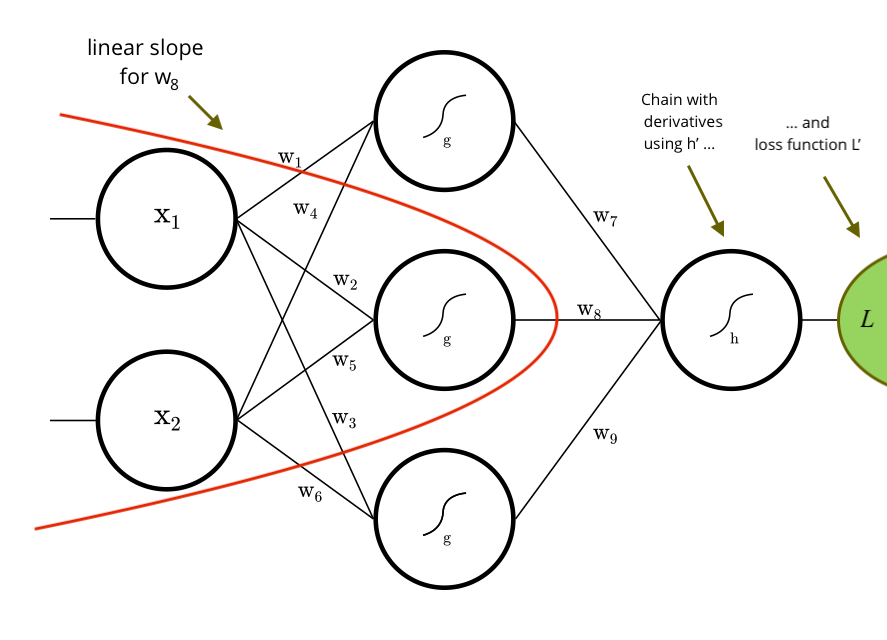
The net above has three layers. On the left, there is the input layer with two neurons. It is simply the raw, untouched input. In the middle we have the Dense layer with three neurons. Here is the area where dots are joined, to learn. The neurons carry Activators and , plain functions, which can be considered as the cells ability to fire. A net can stack many layers, it can be deep. On the right we have the output layer, with one neuron. A net can have multiple input and output neurons, depending on the dimension of our data. The layers are densely connected through synapses, called weights, since the thickness of the synapse determines the amplification between neurons. How to compute the net?
Studying biological neural networks, e. g. nets found in dead animals, it turns out that the connectivity patterns can be modelled through ordinary matrix multiplication. To compute a layer, we multiply inputs by weights and apply the cell's activator to fire. This result is the input of the next layer. If we do this recursively until we reach the output layer, our result is a number, usually between 0 and 1, depending on the activator's domain. This number can be seen as the answer of the net with respect to the given input.
For the sake of brevity, we express this forward pass in matrix notation. The matrices contain the left and right weights coming in and out of the dense layer. Isn't it somewhat calming to know that behind the complex sounding term Artificial Neural Network there is just a couple of matrices and nested function calls?
Training it
If we take our net the way it is, we already can feed it with input and compute a result. But the result would not make much sense, since our net is not trained to recognize bonsais. We need to train it, and we do so by repetition. Let's postulate a numerical representation of a bonsai tree:
A bonsai is a vector or . If I have or it is not a bonsai. Put in equations, we get our training targets :
Supervised training is a repetitive process, for as long as the net is not able to output the labelled targets . Whenever I feed our net with a , I expect it to give 1, and if it is I expect 0 respectively. The difference between expectation and outcome is called Loss. If we look at the big picture, the net in matrix notation, we immediately conclude that the parameters to find in this repetitive process are the weights , because inputs as well as outputs are constant, fixed. It is about the right thickness of synapses, which leads to a minimum loss.
If, and only if, the output of our net equals the target, we know that we have found the optimal weights. The loss would be exactly zero in this case. Since we have four observations, from and , we have to take the sum over these observations, where summands share weights:
Doing some further cosmetics, we finally come up with a nine-dimensional loss function with respect to :
The factor is for convenience when deriving later, and the square gives a convex functional form to not let positive and negative losses neutralize each other, i. e. and we don't want that. This function is called the Squared Error. There are other loss functions, like the Softmax Log Entropy or a Support Vector Machine. For instance, a classification task can have different requirements than a regression task, which results in different formulations of the loss. To train our net we minimize the loss function with respect to the weights:
One could come up with the idea to brute force all nine weights and take the combination leading to the minimum, and it would work, since for a modern computer a nine-dimensional space is fast to brute force. For high resolution data instead, this approach is quickly infeasible, because of a thing called Curse of Dimensionality. What if we have tens of thousands of weights to determine? We would have to try all combinations, which surely takes zillions of years.
We need an analytical approach instead. If we want to know the minimum of a function, we derive its gradients and find a closed form solution with respect to the free parameters. This is done with some straightforward calculus. Deriving the gradients with respect to through a constant application of the chain rule, to tackle the nested activation functions, does the trick. For example, the gradient of with respect to is calculated as follows:
In our ideal mathematical world, all we need was a closed form solution for all to have the true minimum of , but since the real strength of a neural net is learning arbitrary non-linearities, we use non-linear functions for activators and , often in high dimensional spaces with many samples, which leads to complex terms and combinatorial issues, so finding this closed solution is intractable. Since our objective is convex because of the square, an alternative is to come close to the true minimum of by iteratively subtracting our analytical gradients from , stepping downhill towards it. This approximation technique is called Gradient Descent.
The learning rate , usually a small number less than 1, is to be stepping without overshooting and usually is determined using test runs, choosing a small subset of the training data. The size of the subset is called Batch Size, where On-Line means one sample per batch, Full-Batch all samples in one batch and Mini-Batch something in between (M:N). In other words, the training process is a paddle wheel, rolling over all samples, and we control the size of the wheel and update weights after each full loop.
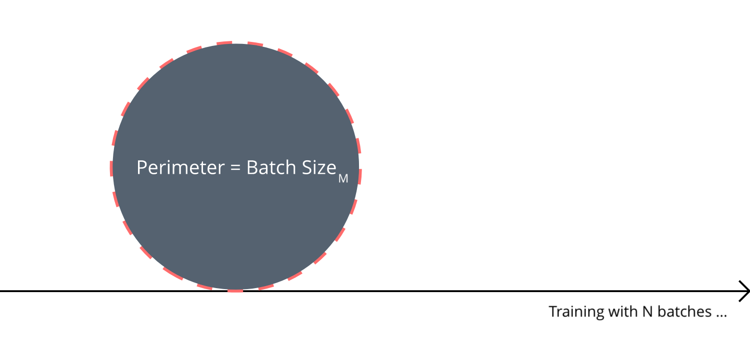
In theory, a full batch is more precise, yet more prone to adjusting dynamically during training, to soften or amplify gradients varying in intensity over time. When training data is grouped into batches, each batch contributes to the minimum of per iteration. Since Big Data implies a certain degree of redundancy, in practice, using mini-batches often gives fast convergence and a more stable . Further, memory and performance considerations arise regarding a good batch size. One important factor is to combine both training data and weights as much as possible using large batches, leading to densely packed matrices. This way the inherent parallelism of a feed forward net can be fully harnessed by multicore processors, on both CPU and GPU.
However, since this is a rather informal blog post, I don't want to go deeper into the mechanics here. If you are curious how the analytical gradients can be constructed algorithmically for batched gradient descent, have a look at NeuroFlow for Scala. Personally, I find functional code easier to understand things than with curly LaTeX math equations. We use this implementation later.
Universal Approximator
Now that we have found a way to train our net, we should be able to recognize bonsais with it. Let's plot the numeric representation of our bonsai tree in two-dimensional space:

The bold points and stand for a bonsai. I picked it on purpose, because you can't separate it linearly. No matter how hard you try, you will never be able to separate and from and using only one line. It is not possible, thus the classification of a bonsai can't be solved through a linear function. Interestingly, our 'bonsai function' is nothing else but the logical XOR function, which formulates binary addition, so we can make our net learn to add modulo 2 as a side effect.
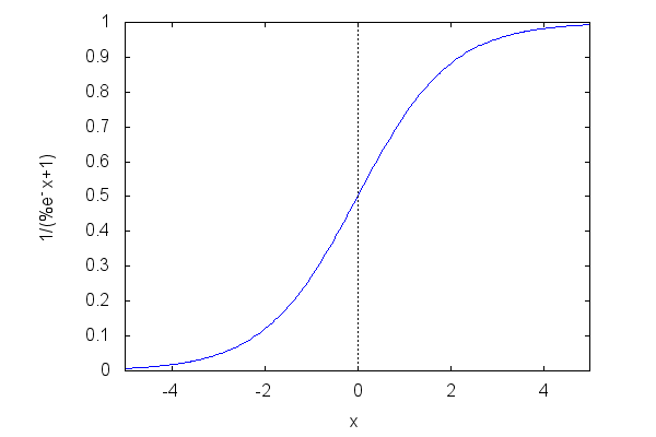
To be an universal approximator, our net must be able to learn such non-linearities, because the patterns we humans produce are most likely non-linear. Looking at our net equation, we immediately conclude that if we insert the linear activator functions and into , we simply get another linear function, since the matrix multiplications won't bring any non-linearity either. Using linear activators, our complex net is not able to recognize bonsais. We can't change the way matrix multiplication is defined, because it mimics the neural connectivity patterns found in nature. Consequently, in order for any neural net to recognize non-linear patterns, we need to find more suitable activators for the cells. There are a few such functions, like Tanh, Sigmoid, or the Rectified Linear Unit. We use the Sigmoid , which is a classic and fits our numeric range .
Because the function depends on the negative natural exponential function as denominator, it is non-linear, and we find a smooth step characteristic, softly firing a neuron, or not.
Now, if we use for and , the net takes the functional form of a nested sigmoid. The complete loss function therefore is:
Theoretically, using this non-linear functional form and gradient descent training, we should be able to separate our non-linear bonsai space.
Let's code it in Scala
  import neuroflow.application.plugin.Notation._
  import neuroflow.core.Activator._
  import neuroflow.core._
  import neuroflow.dsl._
  import neuroflow.nets.cpu.DenseNetwork._

  implicit val weights = WeightBreeder[Double].random(-1, 1)

  val (g, h) = (Sigmoid, Sigmoid)

  val net = Network(
    layout = Vector(2) :: Dense(3, g) :: Dense(1, h) :: SquaredError(),
    settings = Settings(
      learningRate = { case (_, _) => 1.0 },
      iterations = 2000
    )
  )
Now we have a net, initialized with random weights between -1 and 1, a learning rate and maximum iterations for gradient descent. When no batch size is defined, the net assumes a full one. Then, we define the training data using inline vector notation and start training:
  val xs = Seq(->(0.0, 0.0), ->(0.0, 1.0), ->(1.0, 0.0), ->(1.0, 1.0))
  val ys = Seq(->(0.0), ->(1.0), ->(1.0), ->(0.0))

  net.train(xs, ys)
... ah, time for a fresh cup of sencha ...
               _   __                      ________
              / | / /__  __  ___________  / ____/ /___ _      __
             /  |/ / _ \/ / / / ___/ __ \/ /_  / / __ \ | /| / /
            / /|  /  __/ /_/ / /  / /_/ / __/ / / /_/ / |/ |/ /
           /_/ |_/\___/\__,_/_/   \____/_/   /_/\____/|__/|__/
                                                              1.5.6


              Network : neuroflow.nets.cpu.DenseNetwork

              Weights : 9 (≈ 6,86646e-05 MB)
            Precision : Double

                 Loss : neuroflow.core.SquaredError
               Update : neuroflow.core.Vanilla

               Layout : 2 Vector
                        3 Dense (σ)
                        1 Dense (σ)


  INFO neuroflow.nets.cpu.DenseNetworkDouble - [08.02.2018 13:57:49:216] Training with 4 samples, batch size = 4, batches = 1.
  INFO neuroflow.nets.cpu.DenseNetworkDouble - [08.02.2018 13:57:49:263] Breeding batches ...
  INFO neuroflow.nets.cpu.DenseNetworkDouble - [08.02.2018 13:57:49:803] Iteration 1.1, Avg. Loss = 0,503172, Vector: 0.5031724735606108
  INFO neuroflow.nets.cpu.DenseNetworkDouble - [08.02.2018 13:57:49:823] Iteration 2.1, Avg. Loss = 0,502110, Vector: 0.5021102644775862
  INFO neuroflow.nets.cpu.DenseNetworkDouble - [08.02.2018 13:57:49:824] Iteration 3.1, Avg. Loss = 0,501510, Vector: 0.5015098477591278
  INFO neuroflow.nets.cpu.DenseNetworkDouble - [08.02.2018 13:57:49:825] Iteration 4.1, Avg. Loss = 0,501152, Vector: 0.5011517002396553
  INFO neuroflow.nets.cpu.DenseNetworkDouble - [08.02.2018 13:57:49:826] Iteration 5.1, Avg. Loss = 0,500920, Vector: 0.5009203492807744
  ...
  INFO neuroflow.nets.cpu.DenseNetworkDouble - [08.02.2018 13:58:00:200] Iteration 99999.1, Avg. Loss = 8,66563e-05, Vector: 8.66563188141294E-5
  INFO neuroflow.nets.cpu.DenseNetworkDouble - [08.02.2018 13:58:00:200] Iteration 100000.1, Avg. Loss = 8,66554e-05, Vector: 8.6655441891917E-5
  INFO neuroflow.nets.cpu.DenseNetworkDouble - [08.02.2018 13:58:00:200] Took 100000 of 100000 iterations.

  Network was:
  ---
  5.972841198278272  7.031856941751971   -4.693156686110289
  5.958082325044351  -4.709170682392037  6.984931986901868
  ---
  19.752926278797165
  -14.472887673690817
  -14.474769706032983
Clearly our weights have changed and loss is small, looks like everything worked out. To check if our net can recognize bonsais, we feed it with all inputs:
  Input: DenseVector(0.0, 0.0)   Output: DenseVector(0.009977792013595178)
  Input: DenseVector(0.0, 1.0)   Output: DenseVector(0.9940081702899719)
  Input: DenseVector(1.0, 0.0)   Output: DenseVector(0.9940077326864107)
  Input: DenseVector(1.0, 1.0)   Output: DenseVector(0.0013940967243219436)
As we can see, feeding our net with vectors and leads to a number close to 1, whereas feeding it with vectors and leads to a number close to 0. We finally did it! Our net can recognize bonsais, more, it can add binary numbers modulo two. Another interesting property of our trained net is its plot.
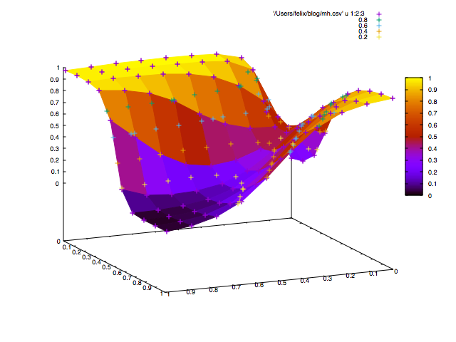
To separate the space, the net draws a mountain landscape, and if we look at the colored surface, we see that only a bonsai gets the peak.
Thank you for reading. :-)