Digit Recognition

Felix Bogdanski, since 13.1.2016

In the [previous article](/blog/natural-trend-detection) we saw how a neural net can be trained to detect trends in two-dimensional charts. Since neural nets are good at learning graphical shapes, this time I want to teach a net to recognize digits from computer typesets, and to generalize to an unknown typeset. You can check the code and data on [GitHub.](https://github.com/zenecture/neuroflow)

Bring me some digits!

Our digits are a very interesting phenomenon, they come in many different varieties. For instance, If we compare several computer fonts, we see that even the _perfect_ ones, those made for screen reading, at times show great variance regarding their shape and style. If we add handwritten sets to our calculation, quickly we realize a lot of shapes can be considered valid, as long as there is a relation to other digits of the set. So, in the end, the neural net not only has to memorize all raw variations, but also learn the subtle connections between the classes.

If we study typesets _a - h_ found in the image above, we see that some of them are similar and some have rather different concepts. The typesets _a, b, c_ and _e_ seem to be similar. Sometimes our brain tries to interpolate between similar typesets, just like a _real_ neural network would do, but if we thoroughly study their shape, we spot the differences. If we train a neural net to recognize a lot of very similar shapes, it will not be able to generalize, so the typesets _d, f_ and _g_ will bring us more variance, where _f_ and _g_ are handwritten sets. The typesets _a - g_ give the training set for our neural net, the last typeset _h_ tests generalization and is not part of the training. I picked the typeset _h_ on purpose, since it is a good compromise between handwritten and computer made sets.

Finding the architecture

Visual recognition brings us the curse of dimensionality quite naturally. While our digits have a low resolution, still each single pixel of a digit contributes to the dimension. A digit has 200 pixels, width and height, multiplied by 3 color channels, so it is 600 neurons for the first layer. Multiplying and adding the neurons of subsequent hidden and output layers, we end up in a high dimensional space, which takes training time and memory for the weights.

Luckily, our digits are relatively fast to train on a modern GPU. For larger images, convolutional nets are used to reduce the neural connectivity. Instead of sensing the whole digit, the net learns simple representations in the convolutional layers, interweaving these using subsequent dense layers. In other words, it extracts features of the input, as insinuated by the image above.

We go with a feed-forward net sensing the whole digit, because of the low resolution. Further, we reduce dimensionality by working with color channels. Let's reduce the color space to a binary representation, 0 for a white pixel and 1 for all other colors, so we shrink the information space from 600 to for each digit.
  
  def digitSet2Vec(path: String): Seq[DenseVector[Double]] = {
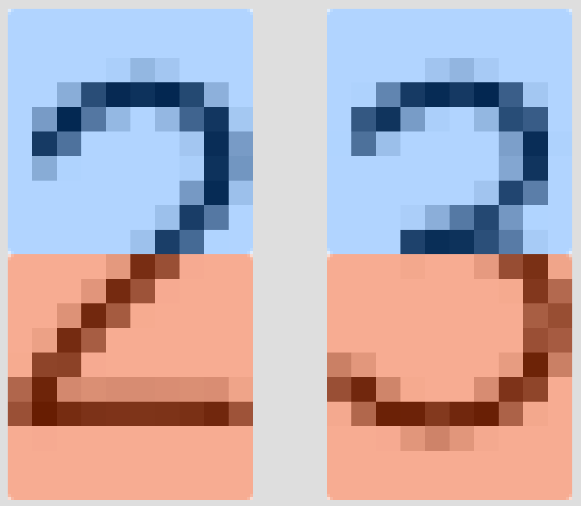
    val selector: Int => Boolean = _ < 255 // Our selector, 0 for a white (255) pixel, 1 for everything else
    (0 to 9) map (i => extractBinary(getResourceFile(path + s"$i.png"), selector)) // Image flattened as vector
  }
  
With layout we should have enough neural connectivity to learn. The input dimension of 200 is determined by resolution, whereas the size of the hidden layers is determined by gut feeling. The output layer has 10 neurons, as we map a digit to one of the possible targets (0-9). Given the predicted scores in range of a digit, our loss function should measure the distance to the true target score, being convex for gradient descent. A target vector is filled with zeros, except for the respective digit to be classified. This is called hot vector encoding, e. g. for digit _2_,

and is to formulate the loss under a cross-entropy regime, i. e. which dimension of represents the true class to maximize the predicted score at by gradient , and to minimize it at for the remaining false classes by gradients . If you are curious how these gradients are derived, I suggest to check out the logarithmic law with respect to , it is a straightforward thing. :-) During training, the predictions in range are generated by , using exponentials to ensure convexity and to softly boost higher raw probabilities normalized such that .

Now if we train digit _2_ with and evaluate, we get a prediction for all ten digits,

each of them interpretable as percent.

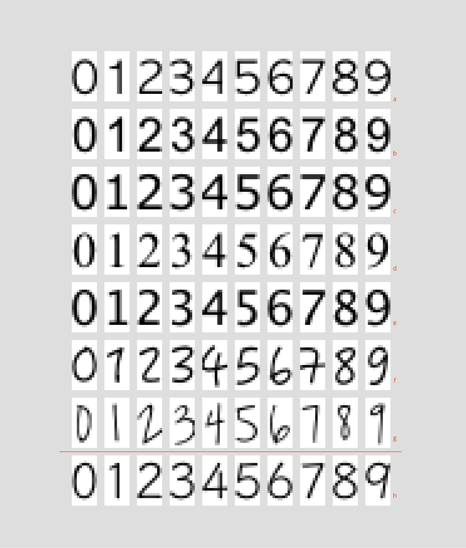
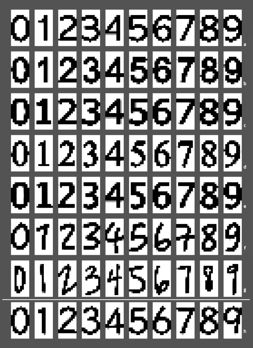
  val sets = ('a' to 'h') map (c => getDigitSet(s"img/digits/$c/"))

  val xs = sets.dropRight(1).flatMap { s => (0 to 9).map { digit => s(digit) } }
  val ys = sets.dropRight(1).flatMap { m => (0 to 9).map { digit => ->(0.0, 0.0, 0.0, 0.0, 0.0, 0.0, 0.0, 0.0, 0.0, 0.0).updated(digit, 1.0) } }

  val config = (0 to 2).map(_ -> (0.01, 0.01)) :+ 3 -> (0.1, 0.1)
  implicit val breeder = neuroflow.core.WeightBreeder[Float].normal(config.toMap)

  val f = ReLU

  val net = Network(
    layout =
      Vector  (200)            ::
      Dense   (400, f)         ::
      Dense   (200, f)         ::
      Dense   ( 50, f)         ::
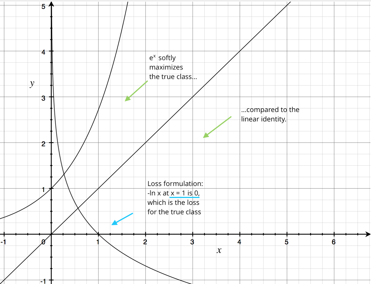
      Dense   ( 10, f)         ::    SoftmaxLogEntropy(),
    settings = Settings(
      learningRate = { case (_, _) => 1E-5 },
      updateRule = Momentum(0.8f),
      precision = 1E-3,
      iterations = 15000
    )
  )

  net.train(xs, ys)
  
Further, we use the [ReLU](http://www.znctr.com/blog/neural-pokemon#relu) activator and _Momentum_ update. _Momentum_ update is a modification of _vanilla_ gradient descent. Instead of stepping, it is jumping downhill into the loss' minimum, iteratively re-gaining momentum into all directions by varying gradients , which is decelerated by factor . Compared to the more gingerly stepping _vanilla_ version of gradient descent, the minimum often can be reached a little quicker.

The first layers consume most of the weights, so we need to initialize their weights smaller by passing _config_ to the weight provider. The weights are drawn from normal distribution, and if you look carefully, you notice that biased weights are produced by normal parameters . This is because the ReLU gets its non-linearity from negative inputs, which can be kinky, because the net will be unable to learn anything if too many weights are negative from the beginning. As soon as a cell turns negative, the ReLU derivative is zero, gradient descent constantly subtracts zero, the cell is dead. Think of a heavy firing brain which needs dead cells to function properly, but not too many of them, so we bias the weights a little to be greater than zero. Alternatively, we could use biased ReLU activators.


       _   __                      ________
      / | / /__  __  ___________  / ____/ /___ _      __
     /  |/ / _ \/ / / / ___/ __ \/ /_  / / __ \ | /| / /
    / /|  /  __/ /_/ / /  / /_/ / __/ / / /_/ / |/ |/ /
   /_/ |_/\___/\__,_/_/   \____/_/   /_/\____/|__/|__/


      Version : 1.3.4

      Network : neuroflow.nets.cpu.DenseNetwork
         Loss : neuroflow.core.Softmax
       Update : neuroflow.core.Momentum

       Layout : 200 Vector
                400 Dense (R)
                200 Dense (R)
                50 Dense (R)
                10 Dense (R)

      Weights : 170.500 (≈ 0,650406 MB)
    Precision : Single


         O
         O
   O     O     O
   O     O     O
   O     O     O     O     O
   O     O     O     O     O
   O     O     O
   O     O     O
         O
         O


[run-main-0] INFO neuroflow.nets.cpu.DenseNetworkSingle - [14.12.2017 17:03:26:824] Training with 70 samples, batch size = 70, batches = 1 ...
Dez 14, 2017 5:03:26 PM com.github.fommil.jni.JniLoader liberalLoad
INFORMATION: successfully loaded /var/folders/t_/plj660gn6ps0546vj6xtx92m0000gn/T/jniloader31415netlib-native_system-osx-x86_64.jnilib
[run-main-0] INFO neuroflow.nets.cpu.DenseNetworkSingle - [14.12.2017 17:03:27:090] Iteration 1 - Loss 0,842867 - Loss Vector 1.3594189  1.0815932  0.06627092  1.2282351  0.40324837  ... (10 total)
[run-main-0] INFO neuroflow.nets.cpu.DenseNetworkSingle - [14.12.2017 17:03:27:152] Iteration 2 - Loss 0,760487 - Loss Vector 1.2405235  1.0218079  0.080294095  1.1119698  0.30945536  ... (10 total)
[run-main-0] INFO neuroflow.nets.cpu.DenseNetworkSingle - [14.12.2017 17:03:27:168] Iteration 3 - Loss 0,631473 - Loss Vector 1.0470318  0.9293458  0.10742891  0.92295074  0.16466755  ... (10 total)
[run-main-0] INFO neuroflow.nets.cpu.DenseNetworkSingle - [14.12.2017 17:03:27:178] Iteration 4 - Loss 0,528371 - Loss Vector 0.8682083  0.8433325  0.17737864  0.7455  0.062339883  ... (10 total)
[run-main-0] INFO neuroflow.nets.cpu.DenseNetworkSingle - [14.12.2017 17:03:27:188] Iteration 5 - Loss 0,439425 - Loss Vector 0.6963819  0.7676125  0.23556742  0.5764897  0.062838934  ... (10 total)
  
Training is done after 15000 iterations or if loss is less than 1E-3, to avoid overfitting.

Let's check

Now that we have a trained net, we need to see if it generalizes:

  ('a' to 'h') zip setsResult foreach { 
    case (char, res) =>
      println(s"set $char:")
      (0 to 9) foreach { digit => println(s"$digit classified as " + res(digit).indexOf(res(digit).max)) }
  }
  
The final classification of one input digit is the output with the highest predicted softmax score. For instance, if we feed our net with digit _3_ of typeset _A_, hopefully, the score for digit _3_ within the resulting vector is the highest. After training and of course a fresh cup of sencha, let's evaluate all sets _A - H:_
Set A
0 classified as 0
1 classified as 1
2 classified as 2
3 classified as 3
4 classified as 4
5 classified as 5
6 classified as 6
7 classified as 7
8 classified as 8
9 classified as 9
Set B
0 classified as 0
1 classified as 1
2 classified as 2
3 classified as 3
4 classified as 4
5 classified as 5
6 classified as 6
7 classified as 7
8 classified as 8
9 classified as 9
Set C
0 classified as 0
1 classified as 1
2 classified as 2
3 classified as 3
4 classified as 4
5 classified as 5
6 classified as 6
7 classified as 7
8 classified as 8
9 classified as 9
Set D
0 classified as 0
1 classified as 1
2 classified as 2
3 classified as 3
4 classified as 4
5 classified as 5
6 classified as 6
7 classified as 7
8 classified as 8
9 classified as 9
Set E
0 classified as 0
1 classified as 1
2 classified as 2
3 classified as 3
4 classified as 4
5 classified as 5
6 classified as 6
7 classified as 7
8 classified as 8
9 classified as 9
Set F
0 classified as 0
1 classified as 1
2 classified as 2
3 classified as 3
4 classified as 4
5 classified as 5
6 classified as 6
7 classified as 7
8 classified as 8
9 classified as 9
Set G
0 classified as 0
1 classified as 1
2 classified as 2
3 classified as 3
4 classified as 4
5 classified as 5
6 classified as 6
7 classified as 7
8 classified as 8
9 classified as 9
Set H
0 classified as 0
1 classified as 1
2 classified as 2
3 classified as 3
4 classified as 4
5 classified as 5
6 classified as 6
7 classified as 7
8 classified as 8
9 classified as 9

Result

Our net architecture is not only able to classify the training digits, but also the generalization test set _H._ Pretty neat!