  def toVector(p: Pokemon): Vector[Double] = p match {
    case Pokemon(_, t1, t2, tot, hp, att, defe, spAtk, spDef, speed, gen, leg) =>
      ζ(types.size).updated(t1, 1.0) ++ ->(tot / maximums._1) ++ ->(hp / maximums._2) ++
        ->(att / maximums._3) ++ ->(defe / maximums._4) // attributes normalized to be <= 1.0
  }
  val xs = pokemons.map(p => toVector(p))
  val dim = xs.head.size // == 23
  import neuroflow.core._
  import neuroflow.core.Activator._
  import neuroflow.core.FFN.WeightProvider._
  import neuroflow.dsl._
  import neuroflow.nets.cpu.DenseNetwork._
val net =
Network(
Vector(dim) ::
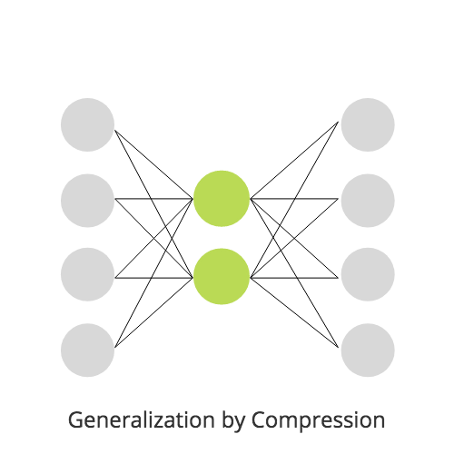
Dense(3, Linear) ::
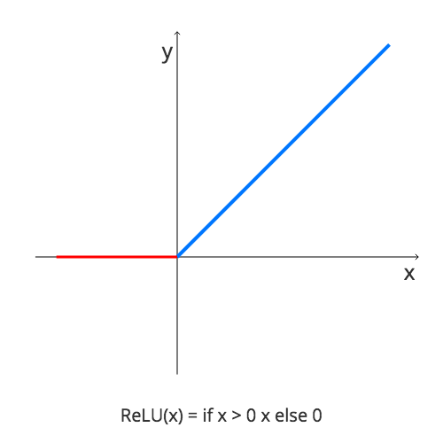
Dense(dim / 2, ReLU) ::
Dense(dim, ReLU) :: SquaredError(),
Settings[Double](
iterations = 5000,
prettyPrint = true,
learningRate = { case (_, _) => 1E-5 }
)
)
net.train(xs, xs)
xs.map(x => net(x))
               _   __                      ________
              / | / /__  __  ___________  / ____/ /___ _      __
             /  |/ / _ \/ / / / ___/ __ \/ /_  / / __ \ | /| / /
            / /|  /  __/ /_/ / /  / /_/ / __/ / / /_/ / |/ |/ /
           /_/ |_/\___/\__,_/_/   \____/_/   /_/\____/|__/|__/


              Version : 1.3.3

              Network : neuroflow.nets.cpu.DenseNetwork
                 Loss : neuroflow.core.SquaredError
               Update : neuroflow.core.Vanilla

               Layout : 23 Vector
                        3 Dense(x)
                        11 Dense (R)
                        23 Dense (R)

              Weights : 355 (≈ 0,00270844 MB)
            Precision : Double


           O                 O
           O                 O
           O           O     O
           O           O     O
           O     O     O     O
           O     O     O     O
           O           O     O
           O           O     O
           O                 O
           O                 O


  neuroflow.nets.cpu.DenseNetworkDouble - [12.12.2017 22:25:26:825] Training with 800 samples, batch size = 800, batches = 1 ...
  neuroflow.nets.cpu.DenseNetworkDouble - [12.12.2017 22:25:27:462] Iteration 1 - Loss 0,984109 - Loss Vector 0.4342741321580766  0.12354959298863942  4.767386946017951  ... (23 total)
  neuroflow.nets.cpu.DenseNetworkDouble - [12.12.2017 22:25:27:508] Iteration 2 - Loss 0,523299 - Loss Vector 0.24434263228748687  0.06230241858166424  2.6454113282008813  ... (23 total)
  neuroflow.nets.cpu.DenseNetworkDouble - [12.12.2017 22:25:27:535] Iteration 3 - Loss 0,371047 - Loss Vector 0.17849810378111158  0.04153676504335314  1.9031709188244275  ... (23 total)
  neuroflow.nets.cpu.DenseNetworkDouble - [12.12.2017 22:25:27:560] Iteration 4 - Loss 0,291979 - Loss Vector 0.14599273484390507  0.0311696796636946  1.500094654118244  ... (23 total)
  neuroflow.nets.cpu.DenseNetworkDouble - [12.12.2017 22:25:27:580] Iteration 5 - Loss 0,242986 - Loss Vector 0.12756149089729327  0.025110515177868865  1.2417398168753926  ... (23 total)
  neuroflow.nets.cpu.DenseNetworkDouble - [12.12.2017 22:25:27:594] Iteration 6 - Loss 0,209563 - Loss Vector 0.11621659294818004  0.021296496834591873  1.0609521279456204  ... (23 total)
  neuroflow.nets.cpu.DenseNetworkDouble - [12.12.2017 22:25:27:604] Iteration 7 - Loss 0,185329 - Loss Vector 0.10858822124655221  0.018846647283148665  0.9273539773987669  ... (23 total)
  neuroflow.nets.cpu.DenseNetworkDouble - [12.12.2017 22:25:27:619] Iteration 8 - Loss 0,167051 - Loss Vector 0.1031596563714349  0.017185307369569098  0.824409293358061  ... (23 total)
  neuroflow.nets.cpu.DenseNetworkDouble - [12.12.2017 22:25:27:632] Iteration 9 - Loss 0,152741 - Loss Vector 0.09916708918647826  0.016068084657543582  0.7421994416221095  ... (23 total)
  neuroflow.nets.cpu.DenseNetworkDouble - [12.12.2017 22:25:27:643] Iteration 10 - Loss 0,141258 - Loss Vector 0.09614992073964508  0.015286892120987623  0.6750032695224172  ... (23 total)
  neuroflow.nets.cpu.DenseNetworkDouble - [12.12.2017 22:25:27:656] Iteration 11 - Loss 0,131864 - Loss Vector 0.09366913014757446  0.014742771731776485  0.619233569973472  ... (23 total)
  ...
  neuroflow.nets.cpu.DenseNetworkDouble - [12.12.2017 22:25:31:023] Iteration 499 - Loss 0,0318495 - Loss Vector 0.06269992174775436  0.017762885408949533  0.034436778622842265  ... (23 total)
  neuroflow.nets.cpu.DenseNetworkDouble - [12.12.2017 22:25:31:026] Iteration 500 - Loss 0,0318402 - Loss Vector 0.0626990056751711  0.01776232163859681  0.03444182413724106  ... (23 total)
  neuroflow.nets.cpu.DenseNetworkDouble - [12.12.2017 22:25:31:026] Took 500 iterations of 500 with Loss = 0,0318402
  [success] Total time: 7 s, completed 12.12.2017 22:25:31
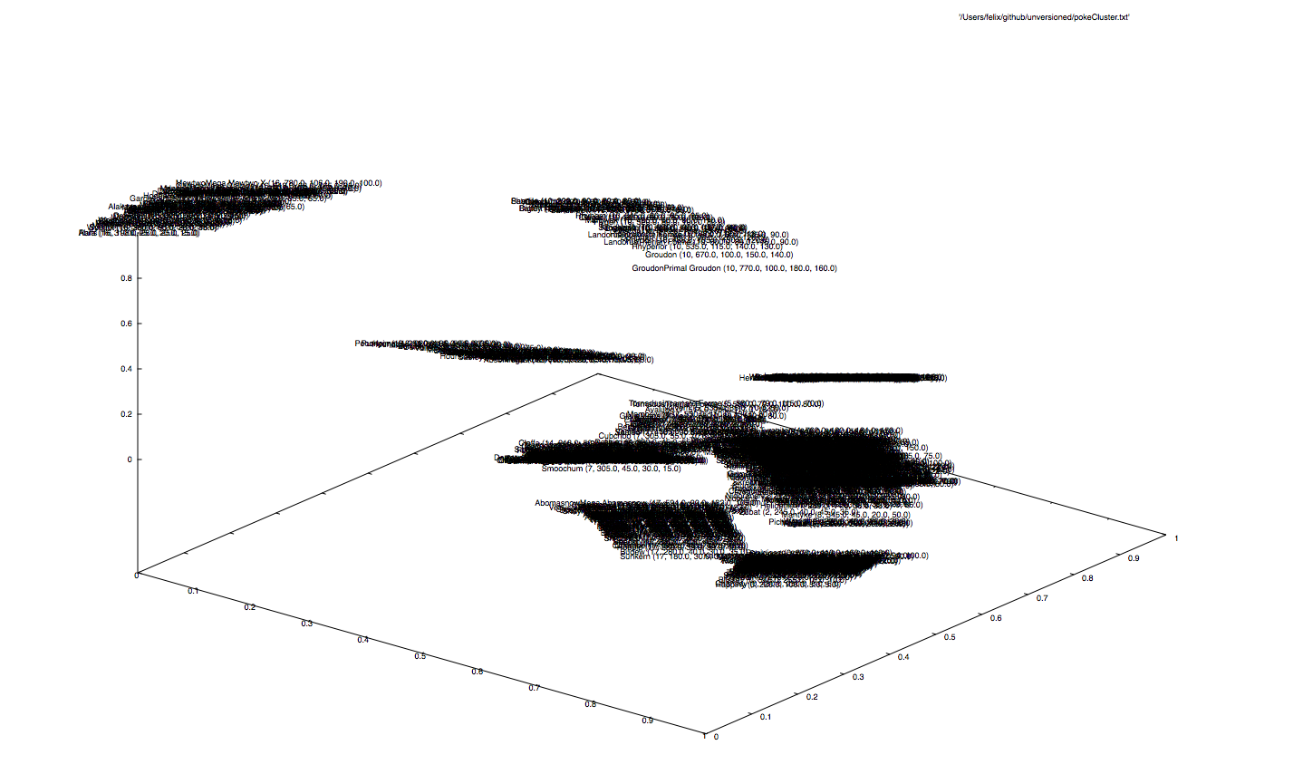
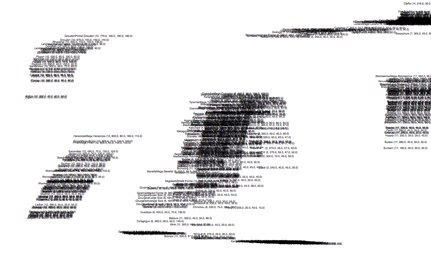
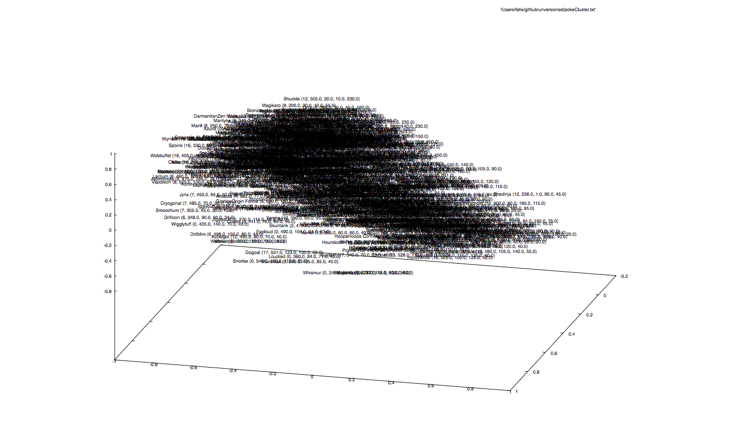
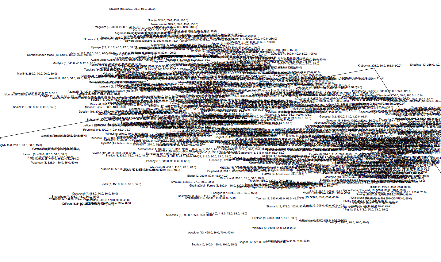
... we find a couple of clusters here. Remember we used five features (type, total, hp, attack, defense), so the net would have to compromise between all 721 monsters.
Some groups are far away from each other, where the attribute type is the dominating clustering key. This comes naturally, because the type is a multi-class vector and contributes to the input vector with 19 (of 23) dimensions. Also, there is a big chunk concentrating at the bottom that is a bit hard to read, since the labels overlap. Eventually, we will discover some kind of numerical ordering in here...
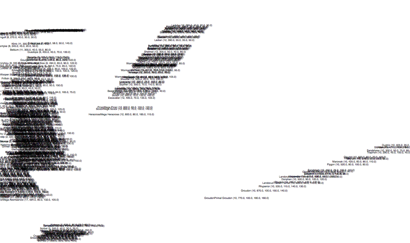
... it seems like the net thoroughly orders the type groups, in such a way, that monsters with higher skills are placed at the top, whereas the ones with lower skills at the bottom (or vice versa, depending on the direction).
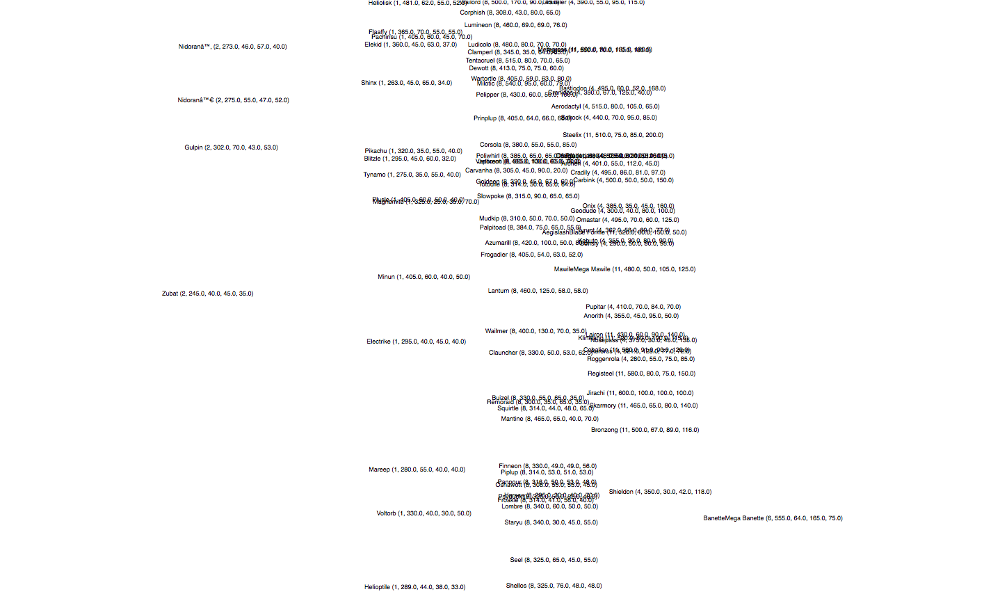
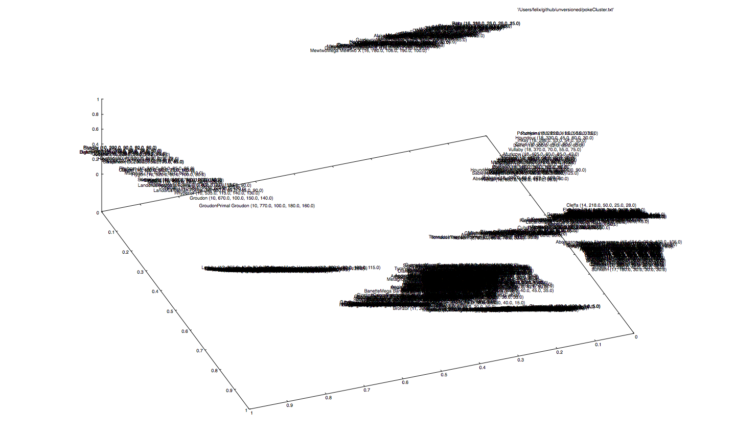
What happens if we remove the dominating feature type, which contributes most to the input dimension, thus giving the net freedom to give up the strict separation between Pokémon types?
... let's see. Mh, it pretty much does the same thing. It places similar Pokémons close to each other. So basically, what we can see is Pokémon2Vec. Note that here we used Sigmoids instead of ReLUs, to add more fuzzyness.