Natural Trend Detection

Felix Bogdanski, at 12.1.2016

In Gaussian vs. Neural Net we compared both, now we research how a neural net can be applied for the detection of trends in 2d spaces. You can check the code and data on GitHub. A trend indicates a lot of people like a certain thing. Possible use cases for detecting trends are stock market, clicks on headlines, social and video platforms, et cetera. When I think of a trend, I see a graph, a steep curve to the top, or bottom if negative. To me, the definition of a trend is a graphical one, thus a good candidate for a neural net, since it learns graphical shapes in a natural way, e. g. neural receptors similar to the human retina.

Looking at the candle bars, we can clearly see an uptrend, supported by the linear function drawn in purple. The green line is a constant, flat function and is the opposite of a trend. How can we train a neural net to differentiate between these two?

Abstract Time Steps

A trend is time, but time is not always a trend. For instance, in the trading scene, a daytrader or scalper is more interested in riding with short term trends, whereas a long-term investor focuses on a much wider timeframe. A long-term downtrend may accumulate a lot of short-term uptrends. Our net should be able grasp the difference bewteen a trend and the complete opposite. We work on abstract time steps, so we can use the net for any time frames. We map the training data to domain , which is for the sigmoid activator. So, as long as input data will be mapped to domain , we can safely use our trained net to detect a trend in time series data of arbitrary length. Let's generate our training data using Scalas Range:


  val trend = Range.Double(0.0, 1.0, 0.01).flatMap(i => Seq(i, i))
  val flat = Range.Double(0.0, 1.0, 0.01).flatMap(i => Seq(i, 0.3))

Here, the trend data is drawn from the linear function from 0.0 until 1.0 with step size 0.01, whereas flat is a constant discrete line. The constant 0.3 is picked arbitrarily and could be marginalized out through a richer training set. Note that choosing, for instance, 0.5 instead of 0.3 leads to similar results. The important thing is that both graphical shapes are clearly separable. Next, we need to spawn a neural network:


  val f = Sigmoid
  val net = Network(Vector(trend.size) :: Dense(25, f) :: Dense(1, f) :: SquaredMeanError())

  net.train(Seq(trend, flat), Seq(->(1.0), ->(0.0)))

We choose a net architecture, with N counting our discrete training values. Every discrete step of our training set will get its dedicated neuron. Plus, a step size of 0.01 means that the range produces neural receptors, so our model lives in a 5025 dimensional space. The output neuron will answer with a number close to 1 if it's a trend, and 0 if it's not. The training succeeds after 118 seconds:


  [INFO] [12.01.2016 12:52:33:853] [run-main-0] Took 61 iterations of 10000 with error 9.965761971223065E-5  
  Weights: 5025
  [success] Total time: 118 s, completed 12.01.2016 12:52:33

Let's see what kind of answers we get for various inputs. Feeding it with training input, a linear and a flat function, we can check if they get classified correctly:


  Flat Result: DenseVector(0.010301838081712023)
  Linear Trend Result: DenseVector(0.9962517960703637)

Yup, good.

Square trend

A pure, linear trend will be rare, so let's try it with a square trend:


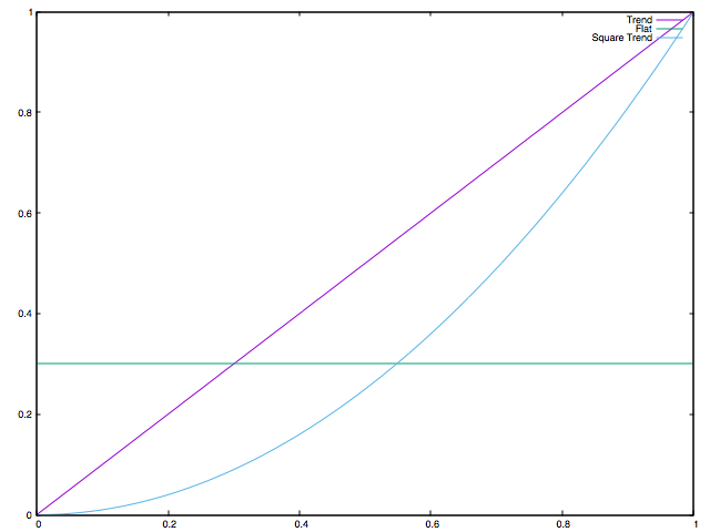
  val squareTest = Range.Double(0.0, 1.0, 0.01).flatMap(i => Seq(i, i * i))


  Square Trend Result: DenseVector(0.958457769839082)

Our net is pretty confident that this is a trend. Check!

Linear downtrend

Let's feed it with a linear downtrend and see what happens:


  val declineTest = Range.Double(0.0, 1.0, 0.01).flatMap(i => Seq(i, 1.0 - i))


  Linear Decline Trend Result: DenseVector(0.0032519862410505525)

Our net is very confident that a linear downtrend is not an uptrend. Check!

Square downtrend

This time, we try a square downtrend:


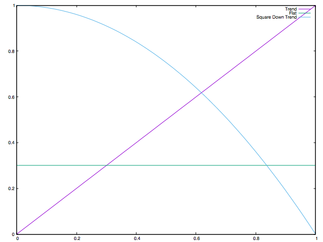
  val squareDeclineTest = Range.Double(0.0, 1.0, 0.01).flatMap(i => Seq(i, (-1 * i * i) + 1.0))


  Square Decline Trend Result: DenseVector(0.011391593430466094)

Our net is very confident that a square downtrend is not an uptrend. Check!

Jamming trend

Let's make it a bit harder and simulate a jamming trend:


  val jammingTest = Range.Double(0.0, 1.0, 0.01).flatMap(i => Seq(i, 0.5*Math.sin(3*i)))


  Jamming Result: DenseVector(0.03840459974525514)

Again, our net is confident that this is not an uptrend. Check!

Hero to zero to hero

What about a curve first being a downtrend, but then recovering to the original level:


  val heroZeroTest = Range.Double(0.0, 1.0, 0.01).flatMap(i => Seq(i, 0.5*Math.cos(6*i) + 0.5))


  HeroZero Result: DenseVector(0.024507592248881733)

Indeed, our net is pretty confident that this is not an uptrend. Check!

Oscillating sideways

Now, we want this oscillating sideways movement to be evaluated:


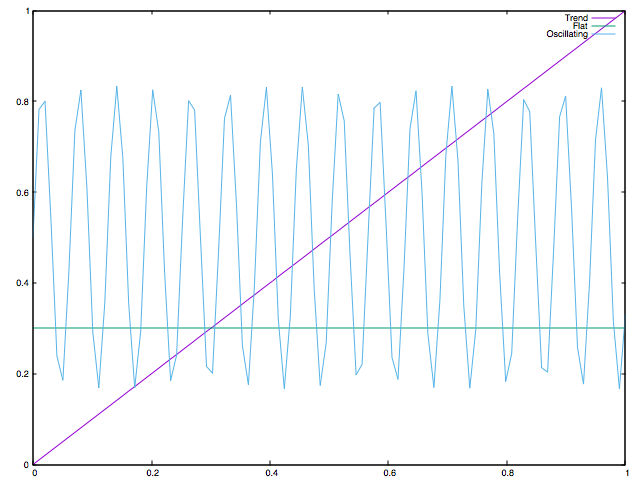
  val oscillating = Range.Double(0.0, 1.0, 0.01).flatMap(i => Seq(i, (Math.sin(100*i) / 3) + 0.5))


  Oscillating Result: DenseVector(0.0332458093016362)

Strike, our net is confident that this is not an uptrend. Check! Let's take a truly random sideways movement:


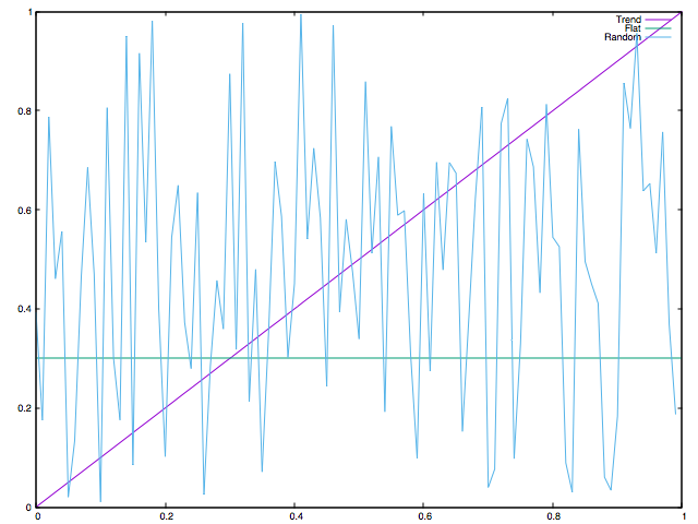
  val random = Range.Double(0.0, 1.0, 0.01).flatMap(i => Seq(i, Random.nextDouble))


  Random Result: DenseVector(0.3636381886772248)

What's interesting here is that our net still says it is rather not a trend - which is correct - but with 0.36 it is not as certain as in the example before. If we examine the range we see a slight uptrend. I guess this is the reason for the increased uncertainty. However, check!

Oscillating uptrend

I want to try an oscillating uptrend:


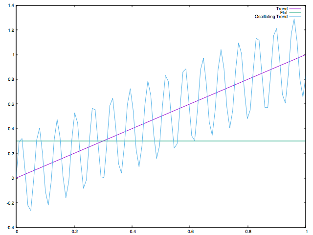
  val oscillatingUp = Range.Double(0.0, 1.0, 0.01).flatMap(i => Seq(i, i + (Math.sin(100*i) / 3)))


  Oscillating Up Result: DenseVector(0.9441733303039243)

Our net is pretty confident that this is an uptrend. Check! But what if we slighty randomize this trend, to make it seem more natural:


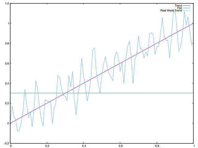
  val realWorld = Range.Double(0.0, 1.0, 0.01).flatMap(i => Seq(i, i + (Math.sin(100*i) / 3) * Random.nextDouble))


  Real World Result: DenseVector(0.9900808890038473)

It's also correctly classified, check!

Oscillating downtrend

Finally, let's try the oscillating downtrend:


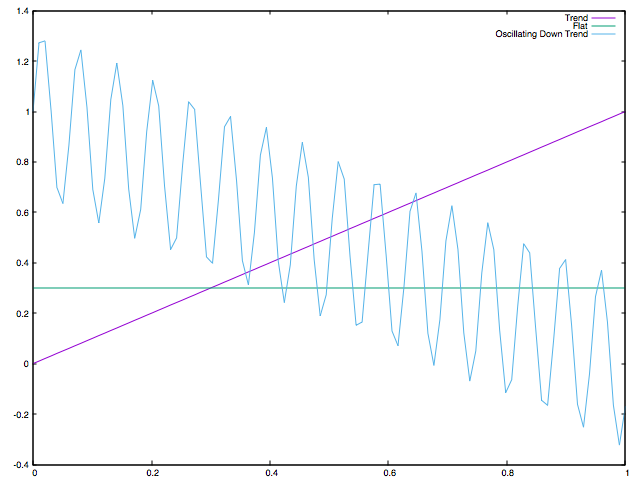
  val oscillatingDown = Range.Double(0.0, 1.0, 0.01).flatMap(i => Seq(i, -i + (Math.sin(100*i) / 3) + 1))


  Oscillating Down Result: DenseVector(0.0030360075614561453)

Again, our net is really confident that this is not an uptrend. Check!

Final thoughts

That's it. We trained a net to detect trends in a timeframe agnostic manner. The extension to more training data to force a stronger generalization is straight forward from here. Also, a multi-output layer is conceivable, so we could detect more states, e. g. uptrends, downtrends and no trends.